
Package room staffing math you can defend: turning daily volume into minutes, headcount, and service targets
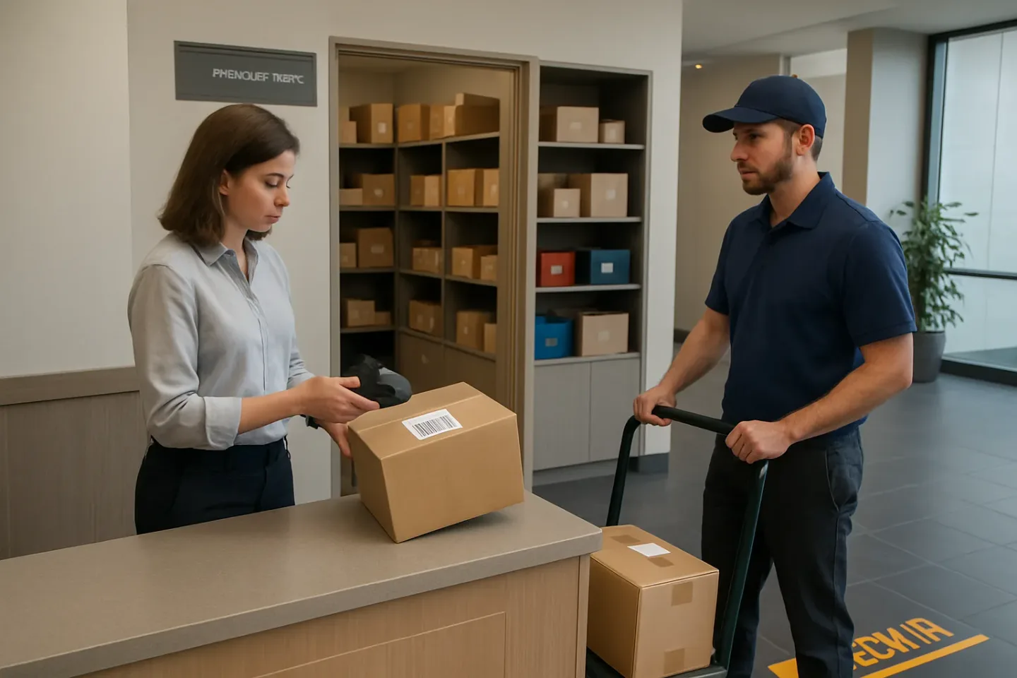
Package room staffing debates often sound like this: “It feels slammed,” “The desk is drowning,” or “We just need one more person.” Those statements may be true, but they are hard to budget, hard to compare across buildings, and nearly impossible to tie to a service promise (like how long carriers wait or how quickly residents get their items). A better approach is a package room staffing model that treats the work as measurable cycle times instead of vibes.
introParagraphs_2_dontuse?placeholder but must be array? -> remove.
introParagraphs_continued? no.
introParagraphs_additional? no.
Define the package room staffing model: three cycle times that explain the work
A package room staffing model works best when it describes the work in a way that is observable, repeatable, and comparable across properties. Instead of arguing about whether a desk team feels “busy,” you measure the minutes it actually takes to complete the same three steps every day, then scale those minutes up or down with volume.
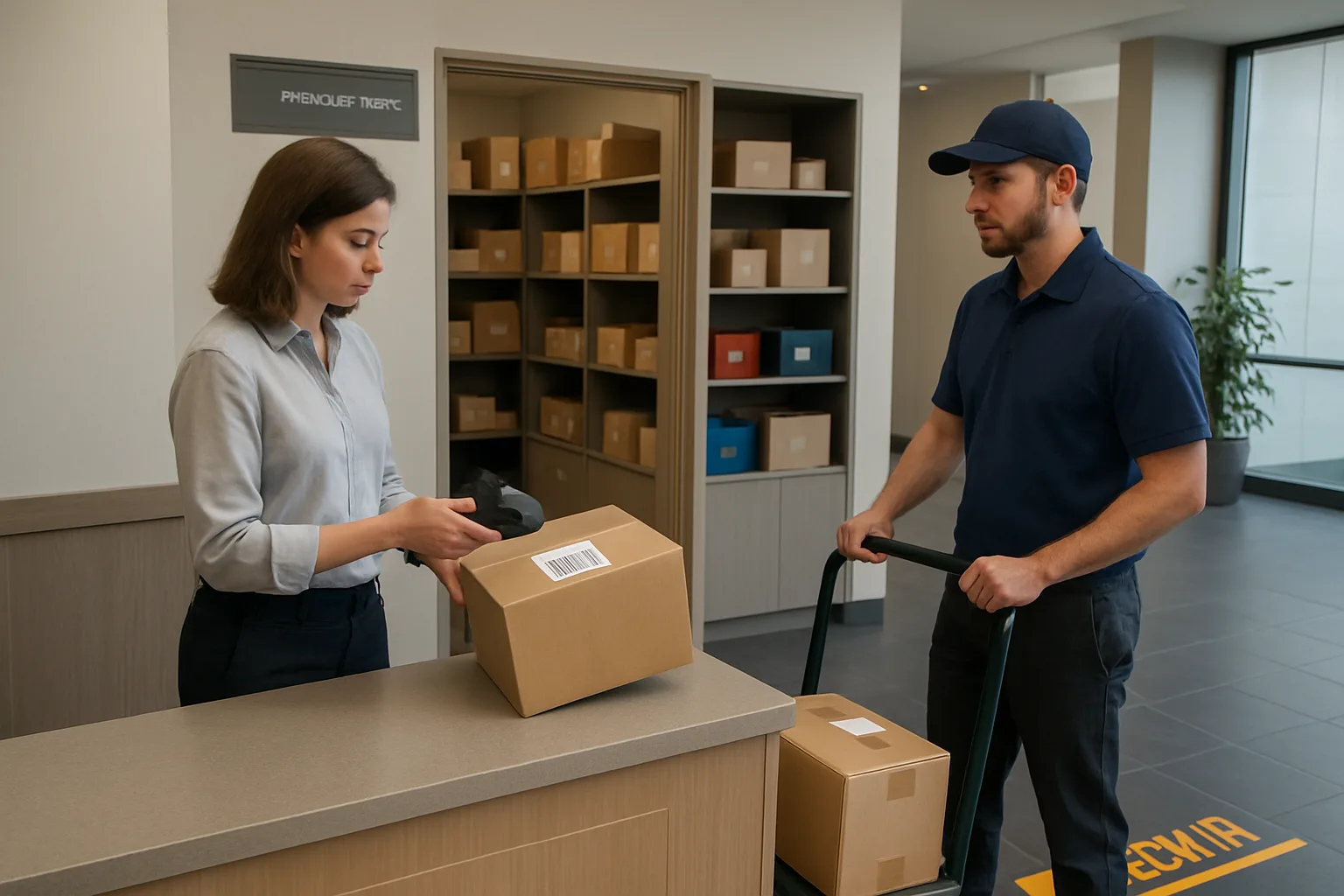
This model uses three cycle times that map to how package work really happens in most buildings: accepting deliveries, putting items away so they can be found, and handing items to residents. If your team measures these consistently (with clear boundaries on what counts and what doesn’t), you’ll have inputs you can defend in budget conversations and operations reviews.
- Model rule 1: Measure what the staff member controls (process time), not what they can’t (carrier arrives early, resident shows up without ID, etc.). Capture those as “exceptions.”
- Model rule 2: Keep cycle times mutually exclusive. Each package should “belong” to one cycle time at a time so you don’t double-count labor.
- Model rule 3: Separate intake work from pickup work. They peak at different times and drive different service targets.
- Model rule 4: Start with averages, but keep a note of variability (range or simple exception rate) so staffing doesn’t collapse on peak days.
Cycle time 1: Carrier check-in (arrival to acceptance)
Definition: The time from when a carrier is ready to hand over packages to when your staff has accepted them and the carrier can leave (or move on). This is the “front door” of your operation and directly affects carrier wait time and lobby congestion.
Start: Carrier arrives at the desk/package room window and indicates they have deliveries (or your staff acknowledges the arrival).
End: Deliveries are accepted and the carrier is released (e.g., signed for, verbally confirmed, or policy-compliant acceptance). The packages may still be on a cart; they do not need to be logged yet for this cycle time to end.
Cycle time 2: Log and store (label/scan, sort, place on shelf)
Definition: The time to convert an accepted package into a findable, accountable item in your system and physical storage. This is where accuracy is created (or lost).
Start: Staff begins processing a specific package or a small batch from the accepted delivery (e.g., picks it up from the intake cart).
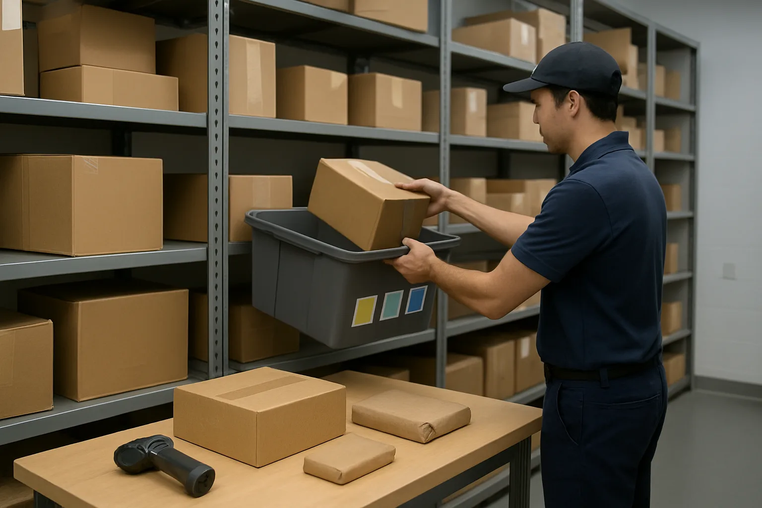
End: The package is logged (manual entry or scan/QR label), assigned to the right resident/unit, and placed in its storage location so another staff member can retrieve it reliably later. If you use shelf zones, this ends when it is placed in the correct zone and any required notification is triggered by your workflow (but avoid timing the resident’s phone/email delivery itself).
Cycle time 3: Resident handoff (locate, verify, release)
Definition: The time to complete a resident pickup from the moment they request their package to the moment they walk away with it (or it is otherwise released per policy). This cycle time drives resident wait time and is often where concierge staffing pressure is felt.
Start: Resident requests a pickup at the desk/package room (in person, via intercom, or other defined pickup flow).
End: Staff locates the correct package(s), verifies the recipient per your policy (unit number, ID check, pickup code, signature), and releases the package(s). If a resident picks up multiple items, time it as a single “handoff transaction” and record the package count separately so you can understand minutes per transaction and minutes per package.
What to include vs exclude (edge cases, oversized items, lockers, after-hours)
You’ll get cleaner data and fewer staffing arguments if you define boundaries up front. The goal is not to ignore messy realities; it’s to track them separately so they don’t distort the core model.
Include (counts toward the cycle time)
Use these as default inclusions so times are comparable week to week:
Carrier check-in: greeting the carrier, directing them to the drop point, quick policy questions, signing/acknowledging receipt (if required).
Log and store: applying a QR label (if used), scanning/typing resident info, resolving simple mismatches (e.g., carrier label shows unit but not name), placing on shelf, updating shelf zone/location if your process includes it as part of storage accuracy. If you do a quick “damage check” or photo as a standard step, include it only if it is required for every package in that category; otherwise mark it as an exception step when it occurs.
Exclude (track as exceptions or separate work types)
Exclude these from the base cycle time so you don’t accidentally bake rare events into everyday staffing assumptions:
Bulk drops: a carrier arrives with an unusually large batch (e.g., 80 packages at once). Record it as a separate observation: same cycle times, but flagged as bulk, because it changes flow and may require temporary staging space.
Bad data: missing unit, illegible label, wrong building, wrong resident, or multiple residents with same name. Time the resolution as exception handling (separately), not inside your normal log/store average. Otherwise you’ll overstaff for errors that could be fixed with process or carrier coaching.
Oversized items and special handling
Decide whether oversized items (furniture, mattresses, multiple-box deliveries) live inside the model or as a separate category. A practical approach:
If oversized is rare, exclude from the base model and track minutes as “special handling” with a weekly count.
If oversized is frequent (common in high-rise move-in periods), create a fourth work type for special handling so you can staff and schedule it explicitly (often with different storage and handoff flows).
Lockers and self-service pickup
If you use lockers or another self-service mechanism, the work doesn’t disappear; it shifts. Adjust definitions rather than forcing locker work into the wrong bucket:
Carrier check-in often stays similar (carrier arrival to acceptance).
Log and store becomes “log and load”: the cycle ends when the package is correctly scanned and loaded into a locker compartment (or staged for locker loading) per your procedure. Count mis-sizes and reassignments as exceptions because they can blow up time unpredictably.
After-hours delivery and pickup
If after-hours deliveries are accepted by security or left in a designated area, avoid mixing those minutes into normal desk cycle times. Instead:
Define a “catch-up intake” work block for the next shift (often a batch log/store session). That block can be measured and forecasted, but it behaves differently from real-time intake during open hours.
For after-hours resident pickups (rare in many buildings), track as exceptions unless it is part of the standard amenity/concierge offering.
Why these three times map cleanly to staffing and service levels
These cycle times translate directly into the questions budget owners and property managers must answer:
How many minutes of labor does inbound volume create today (and next month)? That’s carrier check-in plus log/store.
How many minutes of labor does pickup demand create during peak hours? That’s resident handoff, which is often concentrated in a tight window (evening rush). In other words, you can’t staff pickups using a daily average alone; you need the handoff cycle time and the peak pickup pattern (covered in later steps of the model).
Run a one-week intake time study without disrupting the desk
A credible package room staffing model starts with cycle times you can defend in a budget conversation. The fastest way to get them is a one-week intake time study that is small enough to run alongside normal front-desk work, but structured enough to produce averages and ranges you can trust.
The goal is not a perfect dataset. The goal is repeatable measurements taken the same way, across the same work boundaries, during the windows when staffing pressure actually happens (carrier surges and resident pickup peaks).
- Keep the study lightweight: short observation windows, simple tools, and a clear definition of start and stop points for each cycle time.
- Measure all three cycle times in the same week so the results stay internally consistent (carrier check-in, log/store, resident handoff).
- Capture both averages and spread (typical vs messy) so you can forecast staffing with realistic buffers instead of anecdotes.
Pick a normal week and define the observation windows (peak carriers, peak pickups)
Choose a week that looks like your property most months: no major holiday, no mass move-in day, and no big staffing gaps. If a ‘normal’ week does not exist, pick the closest one and note what was unusual so you can contextualize the results.
Then define short observation windows that match demand patterns. You do not need to time every package all day; you need focused sampling during the periods that drive queues and resident complaints.
A practical setup is to time work in 20- to 40-minute blocks, 2 to 4 times per day, across 5 to 7 days. The key is to intentionally include: the largest carrier arrival period(s), the busiest resident pickup hour(s), and at least one quiet window (to understand best-case speed when interruptions are low).
Sampling targets: minimum counts per cycle time and per shift
Sampling is where most time studies fall apart: teams either measure too little (one hectic hour) or measure so much it disrupts service. Aim for ‘enough to stabilize’ rather than ‘everything.’
Use simple minimums that create credibility without creating a second job. If you run multiple shifts, treat each shift as its own environment because staffing mix, interruptions, and resident behavior often differ.
If you cannot hit these targets in one week due to low volume, extend the study or widen the observation windows rather than accepting tiny sample sizes.
How to measure quickly (phone stopwatch, tally sheet, QR-label scan timestamps)
You can run this study with almost no tools. What matters is that every observer starts and stops the clock at the same moments.
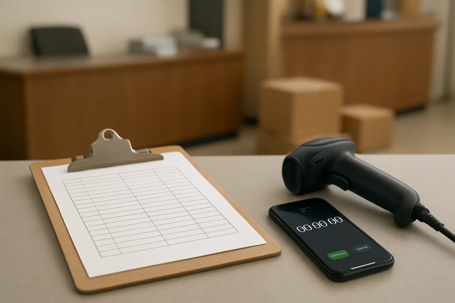
Option 1: Phone stopwatch plus a paper tally sheet. This is the simplest. One person does the work; a second person (or the same person during a quiet window) records times. Write down the duration plus a one-letter code for exceptions.
Option 2: Tally sheet with time buckets. If you cannot stopwatch every transaction, use a 5-minute bucket method during the observation window: count how many check-ins, log/store actions, and handoffs are completed in each 5-minute interval. This yields throughput (packages per hour) directly, and you can later convert to minutes per package by taking 60 divided by packages per hour (for that work type). Keep the work types separate so the math stays clean in your package room staffing model discussion later.
Capture variability: note exceptions (bulk drop, missing unit, broken label, resident forgot ID)
Averages without context get dismissed. Variability notes are what make the numbers believable to budget owners and what help you find process fixes before you ask for headcount.
During each timed event, tag whether it was ‘standard’ or ‘exception,’ and record the exception type with a short code. Keep the list tight so people actually use it.
Examples that commonly swing cycle time in real buildings: bulk carrier drop that requires sorting, missing or invalid unit number, carrier leaves items without a clear recipient, damaged or unreadable label, oversized item that needs a cart or a different storage location, resident arrives without ID or the name does not match, package is misplaced and requires a search, resident requests additional help (bringing items to elevator), access issues (package room locked, dock blocked).
Quality checks: inter-rater consistency and avoiding ‘best behavior’ bias
Two risks can undermine a time study: different people timing differently, and staff unconsciously speeding up because they know they are being measured. Both are fixable with light process.
Inter-rater consistency: Before the week begins, do a 10-minute calibration. Two people time the same 5 to 10 transactions and compare results. If you are more than a few seconds apart on simple transactions, you likely disagree on start/stop points. Re-clarify the definitions and repeat until times are close.
Avoiding ‘best behavior’ bias: Keep observation windows short and varied so the study feels like normal operations, not a performance event. Do not announce a single ‘timing day.’ Rotate who measures. And keep the work rules consistent: staff should follow the usual checklist (label, scan, store location rules, resident verification) rather than skipping steps to look fast. If the process changes during the week (new shelf map, new QR-label routine, new carrier drop procedure), log it; you can still use the data, but you should separate ‘before’ and ‘after’ times instead of averaging them together.
Convert daily volume into minutes and packages per hour (with worked examples)
This is the part that turns a package room staffing model from a discussion into a forecast. Once you have cycle-time averages from your one-week sampling, you can translate any daily volume estimate into total labor minutes and a clear packages-per-hour view for intake and resident pickup. The goal is not a perfect number. The goal is a credible, repeatable calculation you can explain in one page—then adjust as volumes and workflows change.
Below is a simple way to do it without hiding assumptions. You will see each input, each conversion step, and two worked examples you can adapt to your building.
- Key idea: minutes are the universal currency. Volume times minutes per package equals labor demand.
- Separate inbound (carrier check-in + log/store) from outbound (resident handoff). They peak at different times and drive different service targets.
- Use the same cycle-time definitions you measured. If you change what is included, re-measure—do not “adjust in your head.”
Inputs you need: daily inbound volume, pickup volume, percent same-day pickups, open hours
Gather these inputs for the day (or average day) you are modeling. Use your package logs, carrier manifests, or scan counts—whatever your team trusts and can reproduce.
1) Inbound volume (I): number of packages accepted from carriers per day.
2) Pickup volume (P): number of packages handed to residents per day. In steady state, P is often close to I, but it can diverge during holidays, move-ins, or after a weekend backlog clears. Use what actually happens, not what you hope happens.
Inputs (continued): percent same-day pickups and open hours
3) Percent same-day pickups (S): portion of inbound that is picked up that same day. This helps you anticipate whether pickup workload will spike later (backlog). You do not need S to calculate today’s minutes, but it helps validate that your daily pickup estimate is realistic.
4) Open hours (H): number of hours the package room/front desk is open for intake and pickups. If intake can happen while pickups are closed (or vice versa), model those windows separately.
5) Cycle-time averages (in minutes per package), measured from your one-week study: A = carrier check-in minutes per inbound package, B = log and store minutes per inbound package, C = resident handoff minutes per pickup package. Keep the units consistent (minutes/package).
Compute total daily labor minutes for each cycle time
Compute minutes by work type, then sum them. Use these formulas:
Carrier check-in minutes per day = I × A
Log and store minutes per day = I × B (because each inbound package must be logged/stored once)
Compute total daily labor minutes (continued)
Resident handoff minutes per day = P × C
Total package-room labor minutes per day = (I × A) + (I × B) + (P × C)
If you need the inbound and pickup workloads separately (helpful for scheduling), break it out: Total inbound minutes = I × (A + B) and Total pickup minutes = P × C.
Convert minutes to packages per hour by work type (intake vs handoff)
“Packages per hour” is a useful way to communicate capacity to budget owners and desk teams. Once you have average minutes per package, convert to throughput like this:
Inbound packages per hour (intake capacity) = 60 ÷ (A + B)
Pickup packages per hour (handoff capacity) = 60 ÷ C
Throughput interpretation: why this helps staffing conversations
Throughput is not a promise that one person will steadily process that many packages for eight hours straight. It is a clean translation of measured cycle times into a rate stakeholders understand.
Use it to answer questions like: If carriers deliver 120 packages between 4:00–6:00 PM, how many staff-hours are needed in that two-hour window to avoid a line? Or, if pickup surges from 5:30–7:30 PM, how much handoff capacity is required to keep resident wait reasonable?
Worked example: small property (about 60 inbound/day)
Assume your one-week time study produced these averages:
A (carrier check-in) = 0.5 minutes per package (30 seconds)
B (log and store) = 1.5 minutes per package (90 seconds) This could include QR-label printing/affixing, scan, sort, and placing on a shelf/bin location per your checklist.
Small property example (continued)
C (resident handoff) = 1.0 minute per pickup package (60 seconds) This could include locating the package, verifying resident/unit (or ID if required), scanning out, and handing off.
Volumes: I = 60 inbound/day. Pickups: P = 55/day (some items remain overnight). Open hours: H = 12 hours (for context).
Now calculate daily minutes: Carrier check-in minutes = 60 × 0.5 = 30 minutes Log/store minutes = 60 × 1.5 = 90 minutes Resident handoff minutes = 55 × 1.0 = 55 minutes Total = 30 + 90 + 55 = 175 minutes/day (2.9 hours/day)
Small property example: packages per hour view
Inbound capacity = 60 ÷ (0.5 + 1.5) = 60 ÷ 2.0 = 30 inbound packages/hour
Pickup capacity = 60 ÷ 1.0 = 60 pickups/hour
What this tells you: intake work is the “slower” motion here. If carriers tend to arrive in a tight window, staffing should protect inbound intake during that window. Pickup is faster, but can still cause a line if it coincides with interruptions (phone calls, tours, resident questions).
Worked example: high-rise (about 300 inbound/day)
Larger buildings often have different averages because of volume, layout, shelving density, elevator trips to oversized storage, and the number of carriers arriving close together.
Assume these measured averages:
A (carrier check-in) = 0.4 minutes per package (24 seconds) Faster acceptance because the team runs a consistent check-in script and the carrier drop zone is organized.
High-rise example (continued)
B (log and store) = 1.2 minutes per package (72 seconds) Still significant: more scanning/labeling and longer walking paths between zones.
C (resident handoff) = 1.3 minutes per pickup package (78 seconds) Often slower due to searching among dense shelving, verifying multiple packages, and resident questions at the desk.
Volumes: I = 300 inbound/day. Pickups: P = 270/day. Open hours: H = 16 hours (for context).
High-rise example: daily minutes and rate translation
Daily minutes: Carrier check-in = 300 × 0.4 = 120 minutes Log/store = 300 × 1.2 = 360 minutes Resident handoff = 270 × 1.3 = 351 minutes Total = 831 minutes/day (13.9 hours/day)
Packages per hour: Inbound capacity = 60 ÷ (0.4 + 1.2) = 60 ÷ 1.6 = 37.5 inbound packages/hour Pickup capacity = 60 ÷ 1.3 = 46.2 pickups/hour
What this tells you: even with decent per-package times, total daily labor demand is substantial because volume multiplies everything. It also shows where improvements matter most: shaving 0.2 minutes from log/store at 300 inbound/day saves 60 minutes/day immediately.
Add realistic buffers (interruptions, resident questions, access issues) without ‘padding’
Your cycle times already include some “real life” if you measured during normal operations. But there are always tasks that steal attention and break flow—especially when package work is done alongside concierge staffing.
Add buffers explicitly and keep them tied to observable causes. A simple way is to add an allowance factor on top of calculated minutes, then keep a short list of what it covers and how you estimate it. For example: Total adjusted minutes = Total measured minutes × (1 + allowance)
Practical allowance categories you can defend in a budget conversation
Rather than a vague extra 30 percent, document a few common categories you can observe in a week and revisit monthly:
Interruptions: phone calls, resident questions unrelated to packages, vendor entry, key checkouts, tour arrivals.
Exception handling: missing/illegible label, package without unit number, broken box needing re-bagging, carrier wants a signature, resident forgot ID or tries to pick up for a roommate without authorization, package not where the scan says it is (rework).
How to keep allowances honest
Two guardrails keep this from becoming “padding”:
1) Cap the allowance unless you can point to a sustained operational condition. Start small (for example, 10–20 percent) and adjust only if your observations show frequent interruptions or high exception rates.
2) Track exceptions as counts, not stories. If you note that 8 out of 60 inbound packages in a day required relabeling or unit research, that is a measurable driver you can reduce with a better intake checklist or carrier guidance—and you can show the labor savings when it improves.
Turn minutes into headcount and shift coverage tied to service targets
Once you have daily labor minutes for carrier check-in, log/store, and resident handoff, the next step is converting that work into coverage decisions that a budget owner can approve: how many people, for how many hours, at what times, and what service levels you can credibly commit to.
The key shift is to stop treating staffing as a single daily total and start treating it as time-phased demand. Package rooms fail on peaks (carrier clusters, after-work pickup rush), not on averages.
- Goal: translate labor minutes into (1) total hours, (2) peak coverage by hour, and (3) service targets like carrier queue time and resident wait time.
- Core idea: headcount is driven by the busiest 30–90 minutes of the day, not by the daily total.
- Outputs to produce: a staffing plan by hour, plus a clear statement of what waits you can and cannot prevent with that plan.
From total minutes to staffing hours and FTE equivalents
Start with your daily labor minutes by cycle time. Convert to paid hours, then adjust for reality: people take breaks, get interrupted, answer questions, and handle exceptions. Instead of hand-wavy padding, treat this as an explicit utilization assumption (the percent of paid time that can reliably be spent on package tasks).
A simple way to express it is: Required paid hours = (Total task minutes / 60) / Utilization. Many desks operate closer to 0.70–0.85 utilization for package work once you include interruptions and non-package duties that cannot be turned off.
Example: If total package-task time is 360 minutes/day (6.0 hours of pure task time) and you assume 0.80 utilization, required paid coverage is 6.0 / 0.80 = 7.5 paid hours/day devoted to package work. That does not mean one person for 7.5 hours; it might mean two people for 3.75 hours each, concentrated around peaks.
Coverage math: aligning labor to carrier arrival curves and pickup peaks
Daily totals do not tell you whether a single person can keep carriers moving at 11:00–13:00 or keep resident pickup lines reasonable at 17:00–19:00. To schedule coverage, map demand by hour (or by 30-minute blocks) using what you already observe: carrier arrival clusters and resident pickup rushes.
Practical approach: for one representative week, tally inbound drops by hour and resident handoffs by hour (a simple tick-mark sheet works; scan timestamps work even better if you already capture them). Then apply your measured cycle times to each hour’s volume to estimate labor minutes needed in that hour.
Hour-level required headcount is: Headcount needed in hour h = (Minutes of work required in hour h) / 60. Then round up based on service targets (because running at exactly 1.0 headcount leaves no slack for variability). If your 17:00–18:00 window requires 78 minutes of handoff work, that is 1.3 people. In practice, that likely means 2 people for at least part of that hour, or a dedicated ‘pickup runner’ to keep the line moving while the desk continues other duties.
Service targets: defining acceptable carrier queue time and resident wait time
Service targets make staffing math actionable. Without targets, every conversation becomes ‘we need more help’ vs ‘do more with less.’ With targets, you can show what the current schedule can realistically deliver and what would change with added coverage or a process tweak.
Define two simple targets tied to the work you measured: (1) carrier queue/turnaround time during inbound peaks (arrival to acceptance), and (2) resident wait time during pickup peaks (resident arrival to release). Keep them operational and observable; avoid vague goals like ‘fast’ or ‘reasonable.’
Then pressure-test whether your peak coverage can meet those targets. If one associate can complete carrier check-in plus log/store for the inbound burst volume without creating a backlog that spills into resident pickup time, your carrier target is feasible. If not, you either add overlap coverage at inbound peaks or change the intake flow (pre-labeling, batching, staging) so the effective cycle time drops or becomes less variable.
Simple scenario planning: ‘same headcount, different process’ vs ‘more headcount’
Once the schedule is expressed in minutes-by-hour, you can do straightforward scenarios that feel credible in budget discussions because the inputs are measurable.
Scenario A: same headcount, different process. Example levers: pre-print QR labels for common carriers, standardize shelf zoning so storage is faster, use a two-step intake (quick accept + later detailed log) when carriers flood the desk, or add a pickup checklist that reduces rework (wrong shelf searches, mis-scans). In the model, these show up as lower cycle times or lower exception rates, which reduce minutes at the exact peaks that hurt service levels.
Scenario B: more headcount. Add a second person for a narrow overlap window (for example, 11:00–13:00 inbound and 17:00–19:00 pickup) rather than adding an entire shift. In the model, you are buying peak capacity to hit your queue-time targets. You can present the incremental paid hours and the specific service improvement you expect (e.g., preventing a daily backlog that otherwise pushes handoffs into the evening rush).
Where concierge staffing and package work collide: deciding what gets protected during rushes
In many buildings, the same front-desk team handles residents, visitors, access control, phones, and packages. The failure mode is predictable: package peaks steal attention from concierge responsibilities, or concierge interruptions destroy package throughput, and both groups feel the system is broken.
Make the tradeoff explicit by defining ‘protected tasks’ during rush windows. For example: during a carrier burst, one person is assigned to carrier check-in and intake flow (accept, label/scan, stage), while another maintains the desk for residents and building access. During the evening pickup rush, protect resident handoff flow (locate, verify, release) so the line does not grow, while deferring non-urgent admin tasks.
Operationally, this is just role clarity plus a micro-schedule: who is primary for intake, who is primary for handoff, and what gets paused for 30–60 minutes. The model helps you justify that decision because you can show that mixing tasks during peaks increases cycle-time variability (more interruptions) even if the daily total minutes look manageable. Protecting one flow at a time often improves service levels without increasing total headcount—until volume grows beyond what role-splitting can absorb.
Build a credible monthly forecast and keep it accurate
A package room staffing model only helps if it stays anchored to what actually happens in your building. The good news: once you’ve captured one solid week of cycle times, monthly mailroom labor planning becomes a lightweight routine. The goal is not a perfect prediction; it’s a forecast you can defend, update, and connect directly to service targets (carrier wait, resident wait, and same-day availability).
Use this section as a monthly cadence: refresh volume assumptions, sanity-check cycle times, review a small set of operational dashboards, and apply decision triggers before the desk is underwater.
- Keep the model stable: update volume monthly, re-sample cycle times only when something changes.
- Forecast in ranges, not a single number: typical day vs peak day staffing needs.
- Tie every staffing request or process change to a measurable service target (minutes of queue, hours-to-shelf, minutes-to-handoff).
Monthly volume forecast: using recent daily averages and known events (move-ins, holidays)
Start with volume because it changes more often than cycle times. For most properties, you can forecast next month’s inbound packages and resident pickups well enough using a few simple inputs, then let the cycle-time math convert that into labor minutes.
A practical approach is to forecast by day-of-week because package volume is rarely flat across the week. If you do nothing else, separate Monday (or post-weekend) from midweek, and separate Friday from the rest.
What to do each month: (1) pull the last 4–6 weeks of daily inbound counts and daily handoff counts, (2) compute averages by day-of-week, (3) adjust for known events that reliably shift volume, (4) pick a “typical day” and a “peak day” for staffing conversations. Peak day is what protects service targets when things get busy; typical day prevents overstaffing.
Updating cycle times: when to re-sample (process change, staffing change, layout change)
Cycle times should be treated like unit costs: stable until you change the work. Re-sampling every month can create noise and encourage ‘measurement fatigue.’ Instead, re-sample on triggers.
Re-sample (a short, focused study is enough) when any of these happen:
– Process change: you introduce QR-labeling, change the check-in script, add a staging step, or switch how you notify residents. Any step you add or remove will move either log/store time or handoff time (sometimes both).
– Staffing change: new team, new training, or a shift in who does package work (front desk vs dedicated runner). Cycle times often improve after a training reset or degrade when the role becomes ‘whoever is free.’
– Layout change: new shelving, different package room access, relocating the desk, or changing where oversized items go. A 20-second walk becomes meaningful at scale.
– Service-level complaints spike: carriers report long waits, residents report slow pickups, or you see more ‘can’t find package’ incidents. That often indicates cycle-time drift or exception/rework growth.
When you re-sample, keep it small and comparable: capture enough observations to represent peak periods (carrier arrivals and pickup rush) and the most common package types. If your building has distinct flows (for example, lockers for small parcels but manual storage for oversized), sample each flow separately so your package room staffing model doesn’t average away the difference.
Dashboards that matter: inbound by day, handoffs by hour, exception rates, rework time
You do not need an elaborate reporting stack to keep the forecast accurate. You need a handful of views that explain why minutes went up or down: volume, timing, and exceptions.
If you’re building a simple monthly dashboard (even in a spreadsheet), prioritize these:
– Inbound packages by day (last 6–8 weeks): highlights day-of-week patterns and unusual spikes.
– Handoffs by hour (or by 2-hour blocks): shows pickup peaks that drive concierge staffing decisions and coverage alignment.
– Carrier arrivals by window (AM/PM or set windows you use): helps you see whether check-ins are bunching (which affects carrier queue time even if total volume is steady).
– Exception rate: percent of items that require extra handling (missing unit, unreadable label, no access to room, oversized that needs alternate storage, recipient not in system). Track this as a count and as time impact if you can.
– Rework indicators: “couldn’t locate” during handoff, relabeling events, or duplicate logs. Rework time silently breaks packages per hour.
Use the dashboard to validate the story your staffing math tells. Example: if inbound volume is flat but staff feels overwhelmed, you’ll often find the shift in timing (more volume in a shorter window) or exception growth (more time per package) is the real driver.
Decision triggers: when to add coverage, add shelving, adjust checklists, or change intake flow
Forecasting is only valuable if it leads to decisions before service levels degrade. Set triggers that are operational, not emotional. The triggers below are intentionally phrased so you can point to data, not anecdotes.
Staffing and coverage triggers (labor):
– Peak window demand exceeds staffed capacity: if your model shows the peak carrier window requires more minutes than you have labor minutes available, carriers will queue. Add coverage in that window or shift non-package tasks away from it.
– Resident wait time target at risk during pickup rush: if handoff minutes in the 2–3 peak blocks exceed coverage, plan a dedicated handoff person (even temporarily) or add a ‘pickup-only’ counter flow.
Process and layout triggers (minutes per package):
– Log/store cycle time drifts upward: consider a tighter intake checklist, pre-printed QR labels, better sort zones, or changing where commonly picked-up items are stored.
– Handoff cycle time drifts upward: improve findability (bin labeling, shelf maps, standard locations for oversized), tighten verification steps so they are fast, and reduce back-and-forth with residents (“forgot ID,” “wrong name,” “not in system”) by standardizing what’s required.
– Exception rate crosses your tolerance: invest in prevention. For example, a carrier check-in script that forces unit confirmation, a “no unit, no accept” policy with a clear exception path, or a quick way to resolve missing unit in the moment.
Space triggers (shelving and staging):
– You routinely run out of shelf capacity during peak days: add shelving, add an overflow zone with clear rules, or change retention/return timing if policy allows.
– Oversized items consume staff minutes disproportionately: create a designated oversized staging spot and a distinct workflow so oversized doesn’t disrupt standard intake.
The key is to treat these as alternatives you can price out in minutes. If adding shelving reduces average log/store time by a measurable amount, your mailroom labor planning can show whether the one-time expense offsets recurring labor or protects service targets without headcount.
Communicating results: presenting assumptions, ranges, and service-level tradeoffs to budget owners
Budget owners don’t fund ‘busy.’ They fund measurable commitments and defensible assumptions. Present your forecast like an operating model: inputs, cycle times, outputs, and the service levels you can (and cannot) hit.
A simple format that works in budget reviews:
– Inputs: forecast inbound per day (typical/peak), forecast handoffs per day (typical/peak), open hours, peak windows.
– Measured cycle times: carrier check-in, log/store, resident handoff (include the week measured and note if it’s current).
– Buffers: list what you included (interruptions, resident questions, access delays) and keep it consistent month to month.
– Outputs: total labor minutes per day by work type, required coverage by peak window, and implied packages per hour.
– Service targets: carrier queue time target and resident wait time target (for example, “carriers cleared within X minutes of arrival windows” and “resident pickup wait under Y minutes during rush”).
Most importantly, show tradeoffs explicitly. If you keep concierge staffing flat, state what happens: longer carrier waits, slower time-to-shelf, or longer resident lines during pickup peaks. If you add a process change instead of headcount, state what must be true: cycle time must drop by a specific amount (for example, reducing log/store by 20 seconds per package) and you’ll re-sample next month to confirm the change stuck.
This is how the package room staffing model becomes a management tool: a repeatable monthly forecast that links daily volume to minutes, coverage, and service-level commitments—without relying on anecdotes or last-minute firefighting.
Frequently Asked Questions
How many time samples do we need for an intake time study to be credible in a budget discussion?
Aim for enough samples that a single weird delivery or a single fast associate does not dominate the average. A practical target is 30 to 50 timed observations per cycle time (carrier check-in, log/store, resident handoff) across the week, spread across at least two different staff members and multiple days. If you can only do a smaller study, collect at least 15 to 20 samples per cycle time and report results as a range (for example, typical = median, plus a 75th percentile for peak planning). The key credibility move is distribution: sample peak periods (carrier bursts and pickup rushes) plus a few normal periods so you are not modeling a best-case hour.
What is a good way to handle oversized items, refrigerators, or bulk deliveries in the package room staffing model?
Do not force oversized and bulk into the same average as normal parcels. Track them as separate categories with their own cycle times and volumes, because they create different work: elevator runs, two-person lifts, staging, and resident coordination. A simple approach is to add a second line item in your model: oversize minutes = (oversize count per day) x (average oversize handling minutes). For bulk drops (for example, 40 packages for one unit or a retailer drop), treat them as an exception batch with a documented time per batch and schedule coverage for the known carrier window when they happen.
How do we prevent the model from underestimating labor because the desk is constantly interrupted?
Add a measured, explicit interruption factor instead of a vague buffer. During your one-week study, note when a timed task is paused for resident questions, phone calls, door access, or key handoffs. You can either (1) measure pure cycle time and then add an interruption allowance (for example, +10 to +20 percent) based on observed pauses, or (2) measure ‘real elapsed time’ from start to finish including interruptions during representative rush periods. Whichever you choose, write it down as an assumption so budget owners see it is grounded in observation, not padding.
How do we translate staffing math into a service target like “carrier wait time under 3 minutes” or “resident pickup in under 2 minutes”?
Tie the target to peak arrival rates, not the daily average. First, determine the busiest 15- or 30-minute window for carriers and for pickups (count arrivals, not just total volume). Then compare that demand to your capacity: capacity per staff member = 60 / average minutes per transaction for that cycle time. To hit a wait-time goal, plan staffing so capacity during the peak window exceeds demand with some margin (for example, 10 to 20 percent). If capacity is below demand, the queue will grow no matter how good the daily total looks, and you will miss the service target.
We have lockers plus a staffed desk. How do we incorporate lockers into packages per hour and headcount?
Separate flows by where the work happens. Lockers usually reduce resident handoff time (fewer counter transactions) but can increase intake time (sorting, loading, troubleshooting failed locker loads). Model it as: (1) staffed handoffs per day x staffed handoff cycle time, plus (2) locker loads per day x locker load cycle time, plus (3) locker exceptions per day x exception resolution time. This keeps the math honest when lockers are full, QR codes fail, or residents still come to the desk for high-value items.
What should we do when different associates have very different cycle times?
Treat it as an operations signal, not a reason to average everything away. Report two numbers: a typical cycle time (median) and a planning cycle time (75th percentile or ‘new-hire average’). Then document the drivers: layout knowledge, checklist adherence, label/scan habits, and how often they need to hunt for packages. If the gap is large, the staffing model can support a process fix (standard shelf map, QR-label discipline, a pick-list routine, a staged intake table) or a training plan. For forecasting, use the planning cycle time for peak coverage and the typical time for base staffing, so service levels do not depend on always having your fastest person on shift.
Build your package room staffing model this month
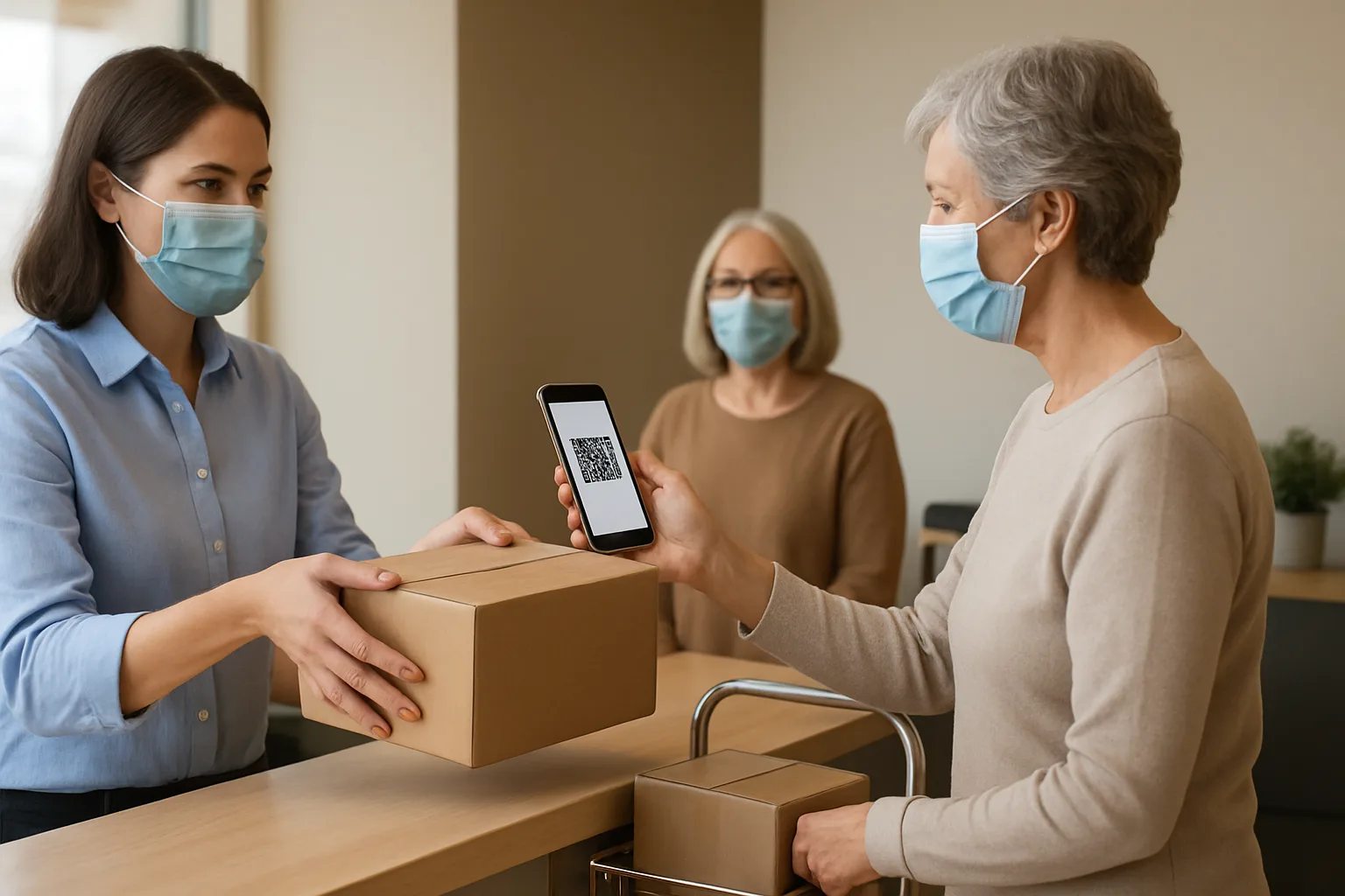
Pick a normal week, sample the three cycle times (carrier check-in, log/store, resident handoff), and convert your daily volumes into minutes and coverage tied to clear service targets. If you want a second set of eyes on your assumptions (what to include, what to exclude, and how to present the tradeoffs to budget owners), TrackNest can help you structure the time study and turn it into a repeatable monthly mailroom labor planning rhythm.
Keep the model alive: re-sample, refresh volume, and use the outputs to make clear tradeoffs
A time-based package room staffing model stays credible because it is grounded in work you can observe: carrier check-in, log/store, and resident handoff. When you sample those three cycle times over one normal week, you get inputs that are defensible in budget conversations and practical for operators who need to schedule the desk. From there, daily volume becomes minutes, minutes become coverage, and coverage connects directly to service targets like carrier queue time and resident pickup wait time.
To keep it accurate, treat the model as a lightweight operating rhythm. Refresh your inbound and pickup volumes monthly, and re-sample cycle times whenever something meaningful changes (staffing experience level, layout and shelving, QR-label workflow, intake checklist, access rules, or a spike in exceptions like missing unit numbers). Track exception and rework notes, not to blame anyone, but to explain why “packages per hour” changed and whether you need process tweaks or additional coverage.
Most importantly, use the model to make tradeoffs explicit. If leadership wants tighter service targets, show the additional minutes (and when they occur). If headcount cannot change, show which process steps must tighten (for example, reducing rework through better labeling/accountability) or which tasks must be protected during rushes so concierge staffing does not quietly absorb package work. When the math is clear, decisions get faster—and your service commitments get easier to keep.